Joint-space Dynamics Library

The jspace library is an easy-to-use model for joint-space dynamics.

It is built on the TAO dynamics engine which allows to compute forward kinematics as well as forward and inverse dynamics of branching structures mode of rigid bodies connected via revolute or prismatic joints.

The best place to start browsing the joint-space documentation is jspace::Model which is the high-level facade that ties it all together.

Trajectory Simulation Application

The trjsim application is an example of how you might use the jspace model: suppose you are given a trajectory and a description of a robot's kinematics and inertial properties. Your task is to determine what the required joint torques and forces would be in order to make joints follow that trajectory.

The trajectory is stored in a text file where each line consists of 2N numbers: the first N numbers are the joint positions, and the second set of N numbers are the joint velocities. Each line represents a sample in time, and the samples are regularly spaced with a fixed timestep.

The robot description is in an XML file that specifies the links and joints, the coordinate frame transformations between them, and their masses and inertias.

The trjsim takes that XML robot file, constructs a jspace::Model from it, and then reads in the trajectory one line at a time. For each sample, it calls jspace::update() with the current state, computes the acceleration required to get to the next sample, and uses the information from jspace::Model::getMassInertia() and jspace::Model::getGravity() in order to compute the torques. It then writes out the positions, velocities, acceleration, as well as the torque with and without gravity compensation.

Once the trajectory file has been completely processed, trjsim prints out a little help text in case you want to plot the result with gnuplot.

Example 1: moving 1kg up 1m

For example, if we have a unit mass robot that translates along the Z axis, we expect the required force to be equal to the acceleration, plus the gravity force of the mass itself which would be 9.81 Newtons:

   $ cd build/jspace/applications
   $ ./trjsim -s ../../../jspace/examples/unit-mass-pz.xml -i ../../../jspace/examples/trj-1dof-a.txt -o result.txt

We can now look at the result in gnuplot:

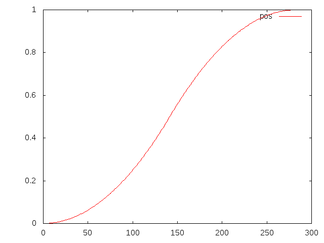
   $ cd build/jspace/applications
   $ gnuplot
   gnuplot> plot 'result.txt' u 0:1 w l t 'pos'
   gnuplot> plot 'result.txt' u 0:2 w l t 'vel'
   gnuplot> plot 'result.txt' u 0:3 w l t 'acc'

example 1 input position

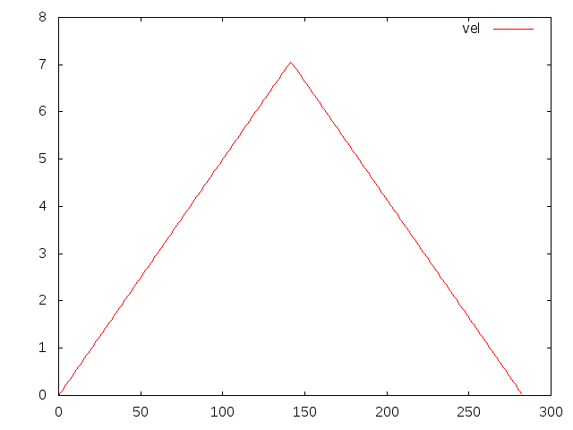
example 1 input velocity

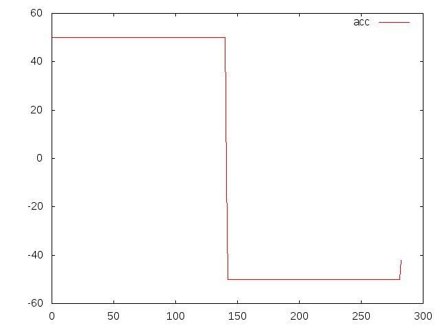
example 1 input acceleration

This shows that the trj-1dof-a.txt example trajectory is a bang-bang control that makes the joint move from position 0 to position 1.

Let's look at the corresponding forces:

   gnuplot> plot 'result.txt' u 0:4 w l t 'tau', 'result.txt' u 0:5 w l t 'tau+g'

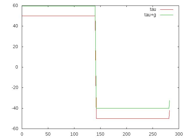
example 1 output

As you can see, the force exactly follows the acceleration.

Example 2: Double-pendulum following a sine-wave

If we have a planar double-pendulum where each arm is 1m long and has 1kg at its end, the situation becomes more interesting for two reasons: the gravity torque will depend on the joint angles, and accelerating one joint will create dynamic coupling in the other. So, we expect the shape of the torques required to follow the trajectory to deviate from shape of the acceleration, and the difference between the torque with and without gravity compensation will not be constant.

   $ cd build/jspace/applications
   $ ./trjsim -s ../../../jspace/examples/unit-mass-rx-rx.xml -i ../../../jspace/examples/trj-2dof-a.txt -o result.txt

We can now look at the result in gnuplot:

   $ cd build/jspace/applications
   $ gnuplot
   gnuplot> plot 'result.txt' u 0:1 w l t 'pos1', 'result.txt' u 0:2 w l t 'pos2'
   gnuplot> plot 'result.txt' u 0:3 w l t 'vel1', 'result.txt' u 0:4 w l t 'vel2'
   gnuplot> plot 'result.txt' u 0:5 w l t 'acc1', 'result.txt' u 0:6 w l t 'acc2'

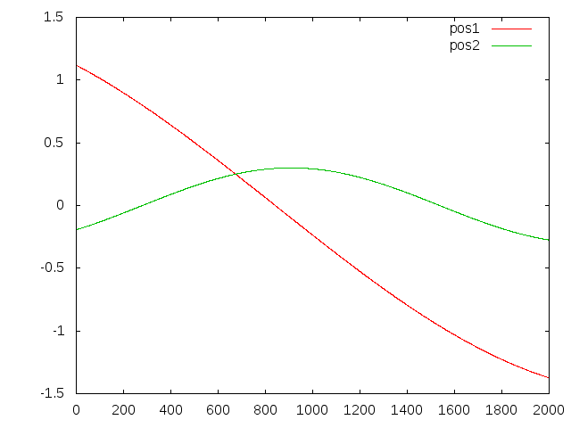
example 2 input position

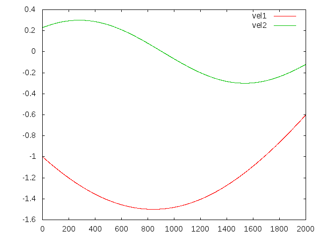
example 2 input velocity

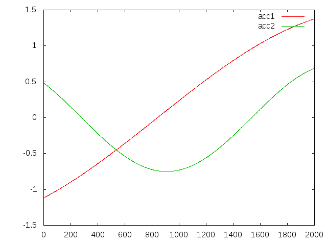
example 2 input acceleration

Here, it will be more interesting to plot the acceleration, torque, and torque+gravity for each joint individually:

   gnuplot> plot 'result.txt' u 0:5 w l t 'acc1', 'result.txt' u 0:7 w l t 'tau1', 'result.txt' u 0:9 w l t 'tau1+g'
   gnuplot> plot 'result.txt' u 0:6 w l t 'acc2', 'result.txt' u 0:8 w l t 'tau2', 'result.txt' u 0:10 w l t 'tau2+g'

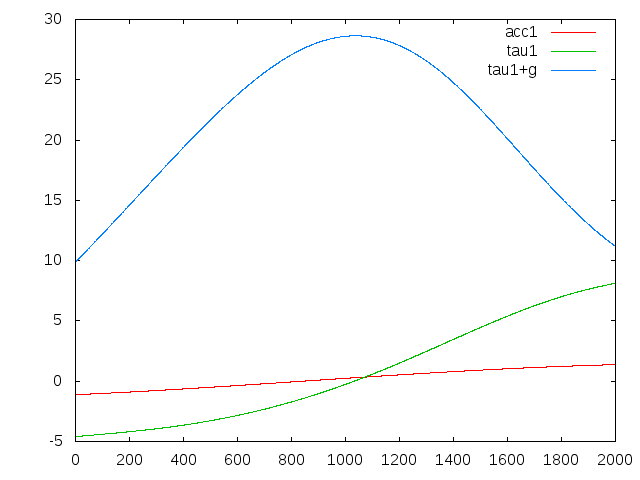
example 2 output for joint 1

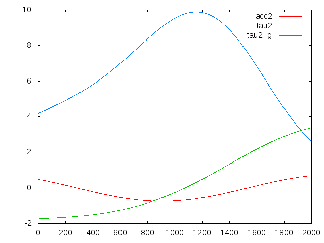
example 2 output for joint 2

This shows that the influence of gravity is quite significant and produces a dependence between the joints. There also is dynamic coupling, but this is not evident in these plots because the accelerations are too low (gravity effects dominate).

---